John Bullinaria's Step by Step Guide to Implementing a Neural Network in C
This document contains a step by step guide to implementing a simple neural network in C. It
is aimed mainly at students who wish to (or have been told to) incorporate a neural network learning
component into a larger system they are building. Obviously there are many types of neural network
one could consider using - here I shall concentrate on one particularly common and useful type,
namely a simple fully-connected feed-forward back-propagation network (multi layer perceptron),
consisting of an input layer, one hidden layer and an output layer.
This type of network will be useful when we have a set of input vectors and a corresponding set
of output vectors, and the aim is for the network to produce an appropriate output for each input it is given.
Of course, if we already have a complete noise-free set of input and output vectors, then a simple
look-up table would suffice. However, if we want the system to generalize, i.e. produce
appropriate outputs for inputs that have never been seen before, then a neural network that has learned
how to map between the known inputs and outputs (i.e. the training data set) will often do a pretty good
job for new inputs as well, particularly if an appropriate regularization technique
has been used.
I shall assume that the reader is already familiar with C, and for more details about neural
networks in general there are plenty of good text-books and web-sites available (e.g., see my
Neural Computation web-site). So, let us
begin...
A single neuron (i.e. processing unit) takes its total input In and computes an associated output
activation Out. A popular activation function is the sigmoid function
Out = 1.0/(1.0 + exp(-In));
/* Out = Sigmoid(In) */
though other functions are often used (e.g., linear or hyperbolic tangent). This
has the effect of squashing the infinite range of In into the range 0 to 1. It also has
the convenient property that its derivative takes the particularly simple form
Sigmoid_Derivative = Sigmoid * (1.0 - Sigmoid) ;
which proves useful when implementing the learning algorithm.
Usually the input In into a given neuron will be the weighted sum of activations feeding in
from the outputs of a number of other neurons. It is convenient to think of the activations flowing
through layers of neurons. So, if there are NumInput neurons in the input layer, the total
activation flowing into a hidden layer neuron is just the sum SumH over all Input[i]*Weight[i],
where Weight[i] is the strength/weight of the connection between unit i in the input layer
and our unit in the hidden layer. Each neuron will also have a bias, or resting state, that is added to
the sum of inputs, and it is convenient to call this Weight[0]. This acts as the
neuron threshold. We can then compute the hidden unit activation with
SumH = Weight[0] ;
/* start with the hidden unit bias */
for( i = 1 ; i <= NumInput ; i++ ) {
/* i loop over input units */
SumH += Input[i] * Weight[i] ;
/* add in weighted contribution from each input unit */
}
Hidden = 1.0/(1.0 + exp(-SumH)) ;
/* compute sigmoid to give activation */
Normally the hidden layer will have many units as well, so it is appropriate to write the weights
between input unit i and hidden layer unit j as an array WeightIH[i][j],
in which we have added the label IH to avoid confusion with any other weights in the network.
Thus to get the activation of unit j in the hidden layer we have
Remember that in C the array indices start from zero, not one, so we would declare our variables as
(or, more likely, declare pointers and use calloc or malloc to allocate the memory).
Naturally, we need another loop to get all the hidden unit activations
One hidden layer is necessary and sufficient for most purposes, so our hidden layer activations
will feed into the output layer in the same way as above.
The code can start to become confusing at this point - keeping a separate
index i, j, k for each layer helps, as does an intuitive notation for distinguishing
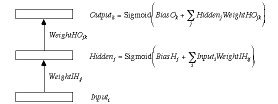
between the different layers of weights WeightIH and WeightHO, the sums of activations
feeding into each layer SumH and SumO, and the resultant activations at each
layer Hidden and Output. The code thus becomes
and the network takes on the familiar form that we shall use for the remainder of this document

Generally we will have a whole set of NumPattern training patterns, i.e. pairs
of input and target output vectors,
{ Input[p][i] , Target[p][k] }
labelled by the index p. The network learns by minimizing some measure of the error
of the network's actual outputs compared with the target outputs. For example, the sum squared
error over all output units k and all training patterns p will be given by
(The factor of 0.5 is conventionally included to simplify the algebra in deriving
the learning algorithm.) If we insert the above code for computing the network outputs
into the p loop of this, we end up with

